Towards the end of 2018, I got engaged (woop!), but that’s not really what this post is about. This post is about the ring.

The ring is designed in OpenSCAD and printed/cast in 14K gold by Shapeways. In the process of designing it, I learnt a whole host of new tricks in OpenSCAD which I wanted to share¹. All of this design work was done in secret, mostly under the guise of “working on my PiWars robot”.

Unusually for me, I’m not going to be sharing full source code or models, because I want this design to stay unique. Hopefully you understand 😄

⚠️ Fair warning: This post is pretty heavy with technical details about the OpenSCAD language, mathematical/numerical operations and programming techniques. If you’re not up for that, perhaps give it a miss! ⚠️

Using hull()

I knew I wanted to make a double-helix ring. My fiancée works in genomic medicine, and a double helix is just plain aesthetically pleasing.

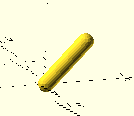
My initial idea was to arrange a set of spheres along the shape of the helix, and then join pairs of the spheres into “sausages” using hull(). Using spheres to make these “sausages”, instead of just plain cylinders, means that where the sausages join the edges are nice and bevelled instead of having sharp corners.

$fn = 16;
hull() {
	sphere(r = 1);
	translate([0, 5, 5]) sphere(r = 1);
}

To turn this into a helix, I deconstructed it into a set of translations and rotations:

1. First translate away from the centre by helix_radius
2. Then rotate around the Z axis by an amount proportional to the distance along the helix
3. Translate along the Z-axis by an amount proportional to the distance along the helix

This needed to parameterised, so I created a module called segment(i = 1) which draws the i^th sausage.

$fn = 16;

helix_radius = 5;
z_step = 0.5;
rot_step = 15;

module segment(i = 1) {
    hull() {
        translate([0, 0, (i-1) * z_step])
            rotate([0, 0, (i-1) * rot_step])
            translate([helix_radius, 0, 0])
            sphere(r = 1);
        translate([0, 0, i * z_step])
            rotate([0, 0, i * rot_step])
            translate([helix_radius, 0, 0])
            sphere(r = 1);
    }
}

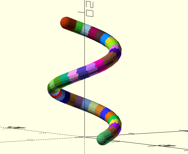
for (i = [1:36]) {
    segment(i);
}

With a random colour assigned to each segment:

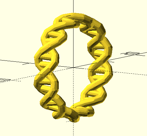
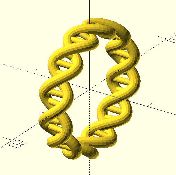
Going from that linear helix to a ring-shaped helix is simply a matter of replacing the final Z-translation with another X-translation followed by a rotation around the Y-axis. Add in a second helix 180-degrees out-of-phase and we’ve got a ring-shaped double-helix:

This was looking pretty nice, so I made some changes to “flatten” the helix in the X direction (I thought that would make a more comfortable ring) and add “bases”, which are just cylinders connecting spheres in opposite strands of the helix.

For the “flattening”, I replaced the first translate() and rotate() with a single translate() using trigonometric functions to position the spheres around a circle (or ellipse, as the case may be). Here, a value of flatten less than 1 will squash the helix in the X direction:

	translate([
		flatten * helix_radius * cos(i * rot_step),
		helix_radius * sin(i * rot_step),
		0
	]) sphere(r = 1);

Everything I’d done so far was using a low $fn value (which is a parameter in OpenSCAD to set the number of edges used to approximate a circle), for speed. This actually gives a pretty cool “low-poly” look, but I knew that wouldn’t survive the polishing process, and so I bumped the $fn…

The render took more than an hour, at a fairly modest $fn setting! That’s totally unacceptable from a development cycle perspective. The long render time is likely due to hull(), which I’ve always found to be a relatively slow operation. At that point I decided I needed a new approach, and went back to the drawing board.

sweep()

I don’t remember exactly where I came across it, but I came across a pair of functions called sweep() and skin() implemented in the list-comprehension-demos of the OpenSCAD repo.

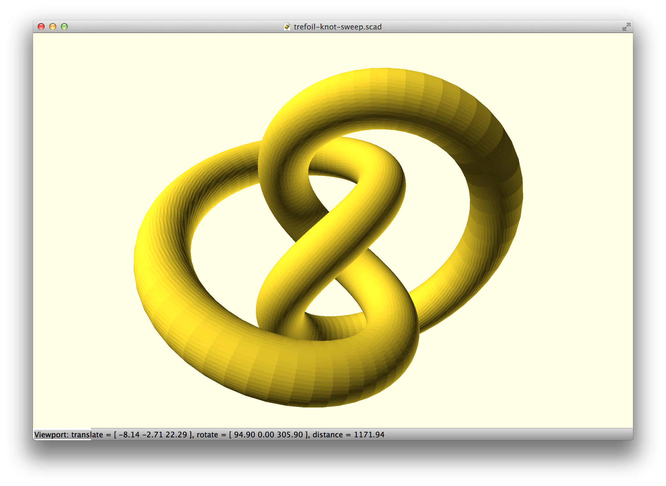
Looking through those examples, the “trefoil knot” looks like exactly the kind of thing I was shooting for.

The way sweep() and skin() work has really opened my eyes to a new way of working with OpenSCAD. Basically, you construct an arbitrary path (as a list of points), calculate (using library functions) the translation/rotation required to get to each point, and pass those to sweep() which will trace through with a 2D primitive, creating a solid polyhedron as it goes. skin() is almost the same, but the 2D shape can be different on each “slice”.

It’s somewhat similar to my approach with joining pairs of spheres into sausages using hull(), but instead of using native OpenSCAD operations, it joins pairs of 2D shapes by creating faces of a polyhedron, connecting the vertices of the 2D shapes.

The whole process is to programmatically generate the vertices/faces for a polyhedron, and then call polyhedron().

polyhedron(points = sweep_points(), faces = concat(loop_faces(), bottom_cap, top_cap), convexity=5);

This idea of using the OpenSCAD language not to combine primitive solids, but to generate vertices and faces is really powerful, and applicable in many different scenarios. It also teaches you a lot about 3D coordinate maths…

List comprehensions and recursion

Before we dive into the specifics of sweep(), it’s worth talking about two concepts which are going to become very important.

List comprehensions

OpenSCAD is a functional programming language, which means its variables behave more like constants in other languages. A variable holds the same value for the whole of its lifetime², which means for example you can’t build a list by adding an element to it each time you go around a loop.

Doesn’t work in OpenSCAD:

square_numbers = [];
for (i = [0:10]) {
	square_numbers = concat(square_numbers, i * i);
}
echo(square_numbers); // ECHO: []

Instead, we have to use list comprehensions - something that also exists in Python. To get the list of square numbers, we’d need to do this:

square_numbers = [for (i = [0:10]) i * i];
echo(square_numbers); // ECHO: [0, 1, 4, 9, 16, 25, 36, 49, 64, 81, 100]

This is a little tricky to get your head into to begin with, but you soon get the hang of it.

Recursion

The other impact of this is that we can’t, for example, use a loop to add up all those square numbers. Doesn’t work:

square_numbers = [for (i = [0:10]) i * i];
sum = 0;
for (i = [0:len(square_numbers) - 1]) {
	sum = sum + square_numbers[i];
}
echo(sum); // ECHO: 0

Instead, we have to use a recursive function, which calls itself over and over again, making a new sum variable each time, until some termination condition is reached (e.g. the end of the list), eventually returning the result:

function sum_list(list, i = 0, sum = 0) = 
	i == len(list) ? sum :
		sum_list(list, i + 1, sum + list[i]);

square_numbers = [for (i = [0:10]) i * i];
sum = sum_list(square_numbers);
echo(sum); // ECHO: 385

This is made a bit more hard to read by the fact we have to use the x = (is-this-true) ? (value-if-yes) : (value-if-no) syntax, so let’s de-construct that, re-writing it in something a bit more C-like, with comments:

function sum_list(list, i = 0, sum = 0) {
	if (i == len(list)) {
		// We're at the end of the list, so 'sum' is now complete.
		// Return it
		return sum;
	} else {
		// Add the current element onto the current sum, and call
		// ourselves again, incrementing 'i' to move on to the next
		// element
		sum = sum + list[i];
		return sum_list(list, i + 1, sum);
	}
}

Trace this through by hand, for a list with length ‘0’:

sum_list([])
|-> i == 0, sum == 0, because those are the default values
`-> i == len(list), so return sum (which is 0)

How about with one element?

sum_list([3])
|-> i == 0, sum == 0, because those are the default values
`-> i != len(list), so call sum_list([3], 1, 0 + 3) 
    sum_list([3], 1, 3)
    |-> i == 1, sum == 3
    `-> i == len(list), so return sum (which is 3)

And one more time with 2 elements:

sum_list([3, 4])
|-> i == 0, sum == 0, because those are the default values
`-> i != len(list), so call sum_list([3, 4], 1, 0 + 3) 
    sum_list([3, 4], 1, 3)
    |-> i == 1, sum == 3
    `-> i != len(list), so call sum_list([3, 4], 2, 3 + 4) 
	sum_list([3, 4], 2, 7)
	|-> i == 2, sum == 7
	`-> i == len(list), so return sum (which is 7)

You get the idea. With each element added to the list, we add one more nested call to sum_list(). At some point, recursion can get “too deep”, and you can run out of stack space. I think OpenSCAD allows a few thousand recursive calls.

Figuring out how to write whatever you want in terms of a recursive function can be quite a brain teaser, but unfortunately it’s a necessity when trying to do procedural generation things in OpenSCAD.

Using sweep()

Actually porting to use sweep() was relatively straightforward. Instead of using translate() and rotate() on a sphere, you work with vectors and transformation matrices (all handled by libraries). This gives a single function f(i) which returns the i^th point on the path.

Most of the gnarly recursion is already handled by the library functions, all that’s needed is a simple list comprehension to build the path. tangent_path() and construct_transform_path() are part of the sweep.scad library, and they are just used to get the transforms argument for sweep().

use <sweep.scad>
use <scad-utils/linalg.scad>
use <scad-utils/transformations.scad>
use <scad-utils/shapes.scad>

function helix(i) = [helix_radius * cos(i * rot_step), helix_radius * sin(i * rot_step), 0];
function f(i) = vec3(rotation([0, hoop_step * i, 0]) * translation([ring_radius, 0, 0]) * vec4(helix(i)));

// Path to trace
path = [ for (i = [start:end]) f(i) ];

// Calculate the loop-closing segment
lastseg = [path[len(path)-1], path[0]];

// Calculate vectors between the samples (replacing the last one with the closed-loop one)
tangents = concat([for (i=[0:len(path)-2]) tangent_path(path, i)], [tangent_path(lastseg, 0)]);

// Calculate transformation matrices (reference frames) for the path
transforms = construct_transform_path(path, tangents);

// Finally, sweep with a circle
// Note that this circle() function is from shapes.scad, and returns a list
// of 2D points. It is *not* the OpenSCAD built-in circle function
sweep(circle(1.0), transforms, closed = true);

This gave me something, but you’ll notice that towards the left-hand-side it gets a little wonky:

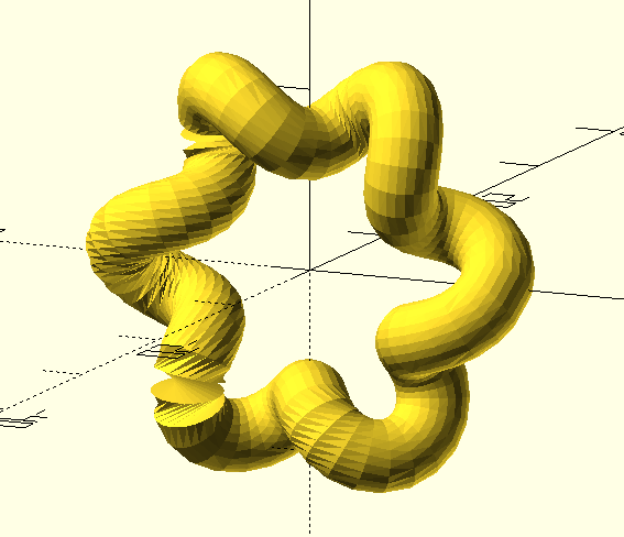
What’s happened here, is a problem with the way sweep() matches up vertices on adjacent 2D slices. In some circumstances, its algorithm picks vertices which aren’t physically close to each other, and you end up with this twisting issue.

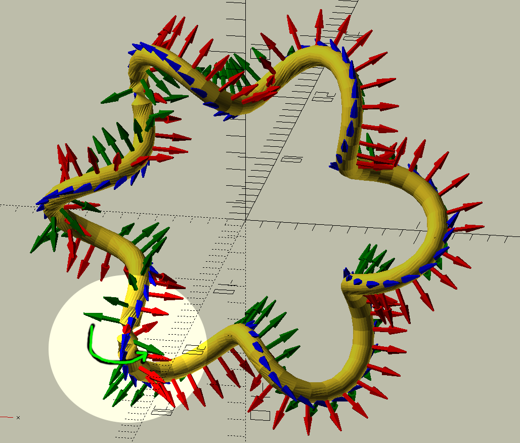
There’s a neat function called frame() in obiscad/vector.scad which draws little 3-axis reference frames, which we can use to visualise the problem. Each of the red/green/blue arrows shows the transformation being applied at each segment of the path. You can see that the blue arrows represent the direction of the path, and the red/green ones trace along the outside like a “spine”. In a couple of places there’s a sudden jump, with the green arrow rotating a large amount around the path in one go. That jump results in twisting in the model:

I found this was a known issue, and spent ages writing my own solution to it; before realising that the forum thread had a second page where someone else had already implemented a superior solution.

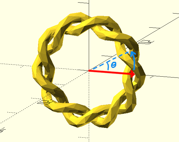
In any case, the fix is to slightly rotate each “slice” around the path (around the “blue arrow”), so that the rotation is spread along the whole sweep() instead of being concentrated at one or two steps. With that fixed, everything was fine³.

A lot more code and refinement later, I had a pretty decent, sweep()-based ring, which rendered in just 1.5 minutes compared to the hour(s) it took using hull().

Setting a stone

I figured an engagement ring needs a diamond, so I needed to find a way to create a setting in my ring. The general theory was to split the helix away from the circle of the ring near the top, and have the four strands form the ‘prongs’ of a prong setting (I made some sketches, but I believe they’ve all been destroyed in the pursuit of secrecy).

But how to describe “organically”-shaped prongs in terms of equations so that I could generate my path points for sweep()?

I decided that Bézier curves were the way to go, and started learning some more maths.

“Bézier” curve sounds scary, but as it turns out it’s pretty straightforward. It’s effectively recursive linear interpolation. For my purposes, I only cared about quadratic and cubic Bézier curves; effectively copying the equations straight off Wikipedia:

function bezier_quadratic(points, t) = let(t1 = (1 - t))
       (t1*t1)*points[0] + 2*t1*t*points[1] + t*t*points[2];

function bezier_cubic(points, t) = let(
       b0 = bezier_quadratic([points[0], points[1], points[2]], t),
       b1 = bezier_quadratic([points[1], points[2], points[3]], t))
               (1 - t)*b0 + t*b1;

function bezier(points, t) =
       len(points) == 3 ? bezier_quadratic(points, t) : bezier_cubic(points, t);

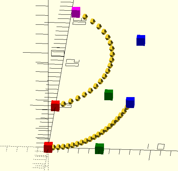
To use the Bézier functions, you give control points (two for quadratic, three for cubic), and a number between 0 and 1 for how far along the curve you are:

quadratic_points = [
	[0, 0, 0],
	[5, 0, 0],
	[8, 0, 5],
];

cubic_points = [
	[0, 10, 0],
	[5, 13, 0],
	[8, 15, 5],
	[2, 10, 10],
];

colours = ["red", "green", "blue", "magenta"];

// Draw coloured cubes for the quadratic control points
for (i = [0:len(quadratic_points) - 1]) {
	translate(quadratic_points[i])
		color(colours[i])
		cube(0.8, center = true);
}

// Draw coloured cubes for the cubic control points
for (i = [0:len(cubic_points) - 1]) {
	translate(cubic_points[i])
		color(colours[i])
		cube(0.8, center = true);
}

// Draw both curves with 20 steps
for (i = [0 : 1/20 : 1]) {
	translate(bezier(quadratic_points, i)) sphere(0.3);
	translate(bezier(cubic_points, i)) sphere(0.3);
}

Armed with these new functions, and a great gemstone model from Kit Wallace on github, I started working on some prongs. You only have to read the commit message to know I was overthinking the problem hilariously:

commit 157cc819faf365abc3cedd9dc488f7e379eaca6a
Author: Brian Starkey <stark3y@gmail.com>
Date:   Mon Jan 15 22:54:19 2018 +0000

    WIP: sink2: Hack together some prongs

    We use beziers to do prongs. Get an intersection in the x/z plane
    between the helix and a vertical prong, and the intersection in the x/y
    plane between the helix and a line parallel to it. Then, bezier through
    them.

Line-plane intersections? What was I thinking?! Look at this insanity, what does it even mean??

function intersect(l1, l2) =
	let( x1 = l1[0][0], y1 = l1[0][1], x2 = l1[1][0], y2 = l1[1][1],
	     x3 = l2[0][0], y3 = l2[0][1], x4 = l2[1][0], y4 = l2[1][1])
	[ ((x1*y2 - y1*x2)*(x3 - x4) - (x1 - x2)*(x3*y4 - y3*x4)) / ((x1 - x2)*(y3 - y4) - (y1 - y2)*(x3 - x4)), ((x1*y2 - y1*x2)*(y3 - y4) - (y1 - y2)*(x3*y4 - y3*x4)) / ((x1 - x2)*(y3 - y4) - (y1 - y2)*(x3 - x4))];

f_on_helix = f(30);
f_on_gem = [1.1 * xtal_x / 2 * sin(45), 1.1 * xtal_y / 2 * sin(45), 9 + xtal_z];
tn_3d = [f(30), f(30) + (f(31) - f(30))];
tn_xz = [[tn_3d[0][0], tn_3d[0][2]], [tn_3d[1][0], tn_3d[1][2]]];
tn_xy = [[tn_3d[0][0], tn_3d[0][1]], [tn_3d[1][0], tn_3d[1][1]]];
prong_down = [f_on_gem, f_on_gem - [0.3, 0, 1]];
prong_xz = [[prong_down[0][0], prong_down[0][2]], [prong_down[1][0], prong_down[1][2]]];
prong_out = [f_on_gem, f_on_gem - [-1, 0, 0]];
prong_xy = [[prong_out[0][0], prong_out[0][1]], [prong_out[1][0], prong_out[1][1]]];
xz_p = intersect(tn_xz, prong_xz);
y_p = intersect(tn_xy, prong_xy);
p0 = f(30);
p1 = [xz_p[0], y_p[1], xz_p[1]];
p2 = f_on_gem;

c = [for (i = [0:20]) let(lint = i * 0.05) bezier(p0, p1, p2, lint)];

So let that be a lesson to you - while programmatically generating paths is powerful, it’s pretty easy to go overboard and write something completely incomprehensible.

Anyway, the result proved that achieving what I wanted should be possible. The basic premise is to put a Bézier control point at the point on the helix where the divergence should start, one at the side of the stone where the prong should finish, and one or two in the middle somewhere to make it look right (bezier control points shown by coloured cubes in the image below):

At this point I had all the tools I needed to simply iterate and polish the ring design (and make the code much cleaner and more sane!) fairly sporadically over the next several months.

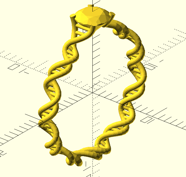
I briefly experimented with a more “biologically accurate” design - it turns out that in DNA the two strands aren’t 180 degrees out of phase. However, the “accurate” one just isn’t quite as pretty, and also looks less comfortable:

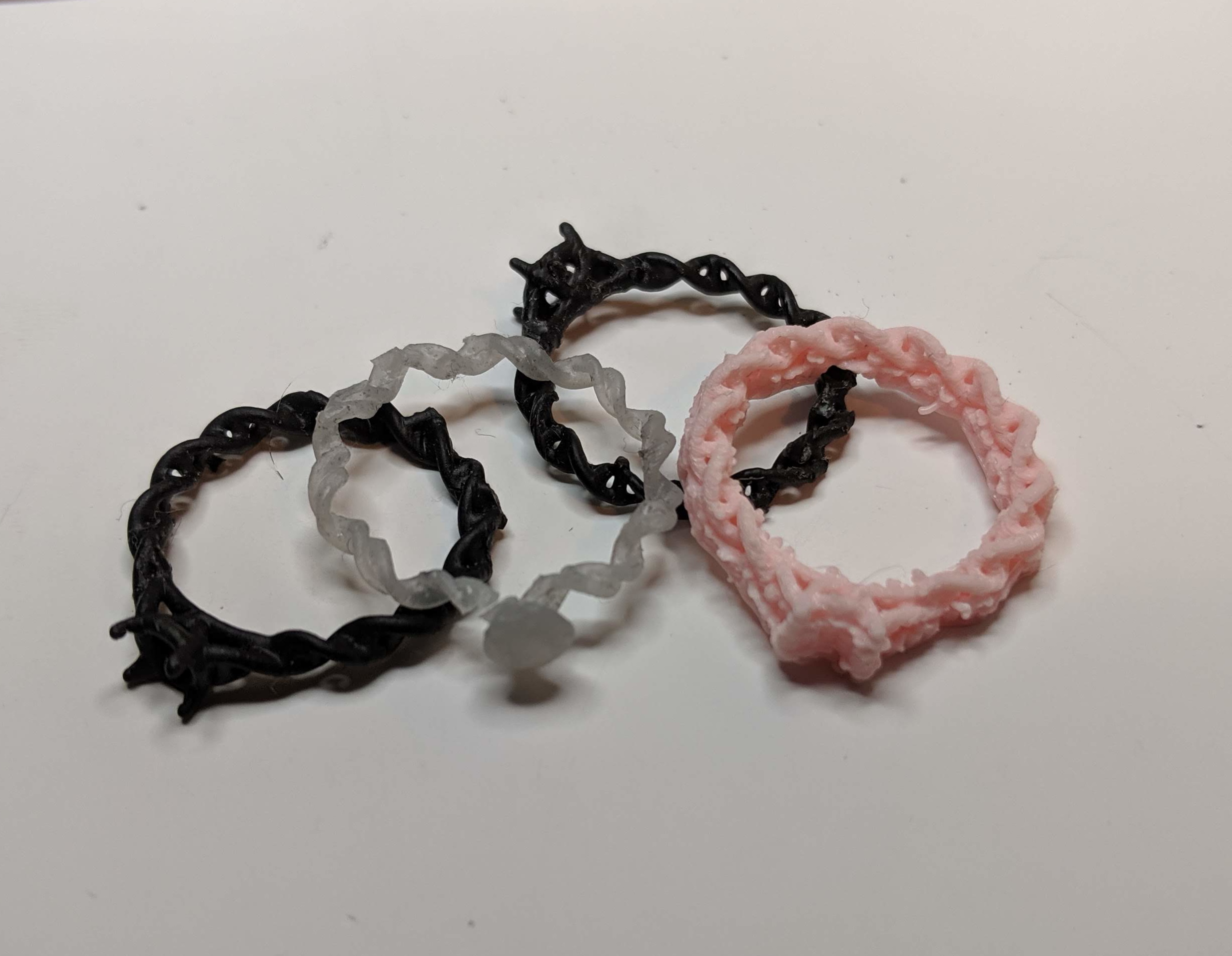
Along the way, I used Makespace’s Form 1+ resin printer (and Ultimaker, unsuccessfully - pink) to print a few different prototypes, because it’s really hard to get a feeling for the physical size of something when you’ve only ever worked on it in CAD.

I did a fair amount of online research into how to make stone settings, to try and figure out what diameter of metal I needed, and how to support the stone. There’s not that much information around, as jewellery making has generally been an artisan craft with 1:1 tutoring and passed-down experience. Still, I eyeballed a bunch of designs and watched a bunch of YouTube and decided that so long as I had some little notches for the stone I’d probably be OK.

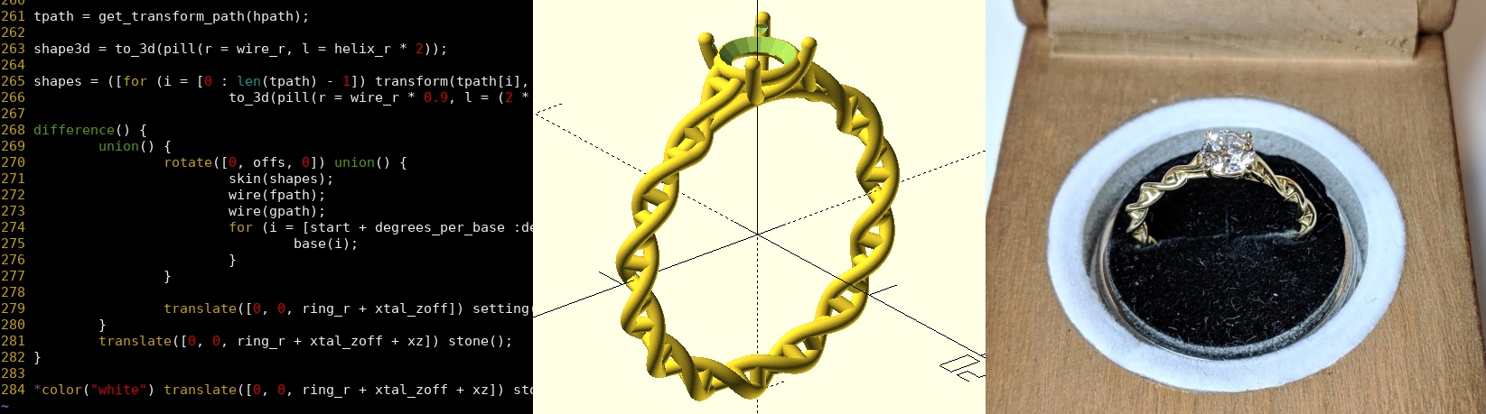
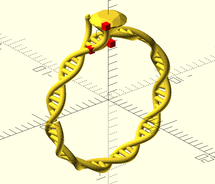
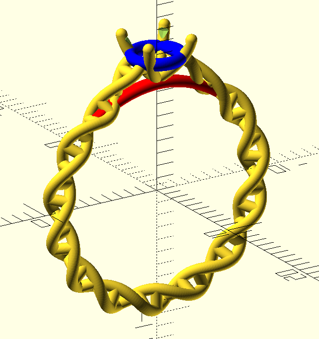
Eventually I settled on the helix not being used for the prongs directly, as the sharp corner required to get the prongs to bend back on themselves always looked ugly. Instead, the helix “diverges” from the ring near the top (forming the “shoulders”), following a Bézier curve up to the “gallery rail” (shown in blue). There, the helix flattens (using the same technique from earlier) to join it neatly.

Underneath the setting, I’ve got a simple smooth “bridge”, made by sweep()-ing a ‘pill’ shape (shown in red). It starts and ends “inside” one of the bases, so the ends are seamless.

The prongs are made using cubic Béziers sweep()-ing a circle, and then capped with a sphere. The control points for the Béziers are positioned with a mix of parametric trigonometry and some fine-tuning by hand.

Sizing, colours and setting stones

If you’ve never tried, surreptitiously finding out the ring size of a long term partner without raising suspicion is a tricky business. I got a best-guess from one of her other rings, but I wasn’t confident enough to go ahead and get the proper gold ring made.

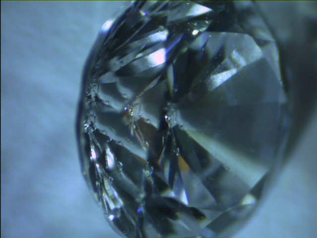
Instead, for the actual asking of the question, I got Shapeways to make a gold-plated brass ring, and bought some 25p cubic zirconia on eBay (because I’m a classy gent). You get what you pay for; under a microscope they’re really chipped and nasty, and look fairly “dull” - presumably as a result of poor cut and polish.

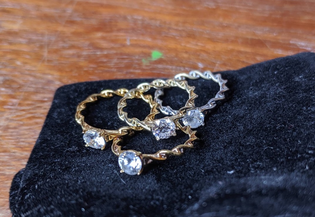
I’m glad I went this route, because it took another two iterations to get the size perfect, and in the process we got a rose gold (plated), yellow gold (plated) and rhodium (plated) ring⁴. When size and colour was settled, I took advantage of a business trip to San Francisco to go to Brilliant Earth to see what loose diamonds look like so I could pick one (because I really had no idea how to pick a diamond, like most people I imagine).

Let me tell you this: Even having practiced with the cubic zirconia on the protoype rings, setting the real diamond into a ring was one of the most nerve-wracking experiences of my adult life. While diamonds are hard they’re also very brittle, and there’s not a whole lot you can learn on the internet about how hard you can squeeze the pliers before you chip the stone. That said, 14K gold seemed much easier to bend than the brass.

The end result is well worth it. The difference in clarity between the rough machine-cut zirconia and the well-cut, well-polished diamond is actually pretty surprising (though not communicated well on camera), and we’re both really pleased with the final ring 😄.

Designing the ring and getting it made was really fun, and I can see myself really getting into it. I can also see it being a real threat to the “traditional” jewellery market. The difference in labour cost is really significant, and the speed of iteration blows the manual techniques out of the water.

So, the next jewellery project (already in progress, and rejected by Shapeways design rules this morning 😢) is to design the wedding rings…

---

1. I also learned that Shapeways' metal printing/casting process is insane! The detail and quality of the pieces is staggeringly good. ↩︎

2. So you can technically re-assign a variable, but it will always hold whichever value was last assigned to it at compile time, i.e. anywhere in the program, even if that assignment comes “lower down” the program than its use. ↩︎

3. There was still one frustrating issue related to CGAL throwing an assertion about non-planar faces, but it has been fixed in recent versions of OpenSCAD. ↩︎

4. The rhodium plating was really bad, and wore off incredibly quickly. I don’t know if that’s a common problem, or we just got unlucky with this one piece. ↩︎