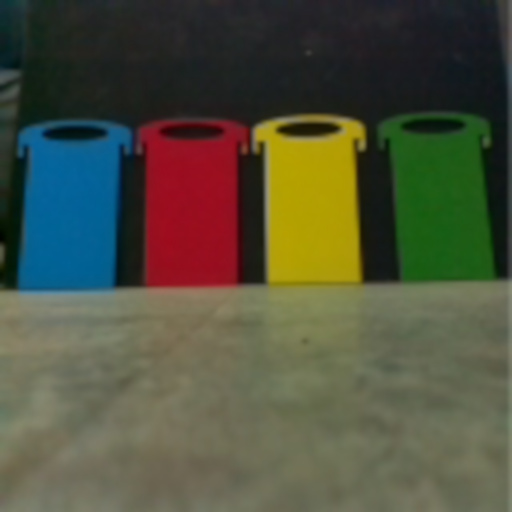
The Hubble Telescope Nebula Challenge (previously Somewhere Over the Rainbow) is one of the autonomous challenges, requiring the robot to visit the four corners of a square arena, starting from the centre. In each corner, there’s a coloured board - and for maximum points the robot must visit the corners in an order specified by their colours (Red, then Blue, Yellow and finally Green), as quickly as possible.

My overall strategy for this challenge is to spin on the spot at the starting position, to identify where each colour is. Once all four corners have been identified, they can be visited in the appropriate order. Originally, I was also intending to use the camera to make sure the ‘bot stays on-course whilst en-route to the corners, and to detect when a corner has been “visited”. Ultimately, I’ve found dead-reckoning using the IMU and counting wheel rotations is reliable enough, and so I’ve skipped the added complexity of using camera feedback for the actual “visiting” phase.

Corner Identification

Phase 1, is to identify where each colour is. For this, I am convinced that the correct approach is to get a sample of the pixel values in all four corners first, and then assign them to colour names, once the pixel values are known for all four. This removes any need for calibration - in all cases, the “blue” corner should be the most blue of the four actual samples. It doesn’t matter exactly what kind of blue it is - only that it’s more blue than all other corners.

The alternative approach, is to assign a corner to a colour as you go - trying to match the pixel value against some expected value for each colour. The problem with this approach, is that it requires calibration (to determine the expected values), and is highly sensitive to things which affect that calibration - such as the lighting conditions, or the quality of the paint finish.

In my implementation, the robot takes a photo once it has turned to face a corner (using the IMU). In theory, the coloured board should then be right in the centre of the camera field of view - however I didn’t want to depend on being able to do a 100% accurate turn. Instead, I use my edge-detection code to look for the vertical lines which represent the left and right edges of the board, and then sample the centre pixel between those lines. This gives me a pretty robust way to get a pixel value for each board.

With a pixel value for each corner, the next task is to figure out which colour is which. One of the key decisions for this is which colourspace to use. You may think that HSV would be the ideal choice, as the relevant information is represented by a single value (hue), however I don’t believe that to be true. Using hue would require taking an observed hue value (from the camera) and comparing it against an expected hue value (from calibration); meaning we’re back to requiring calibration.

Instead, I’m using YCbCr, which can represent the colour as a point on a 2D plane (we can ignore ‘Y’ and use only Cb and Cr as X and Y respectively). This is another advantage versus RGB, for example, where we’d need to use all three component values as coordinates in a 3D space, making classification harder.

The image below shows the “actual” board colours as seen by the camera (sampled from the image above) plotted onto a YUV plane¹:

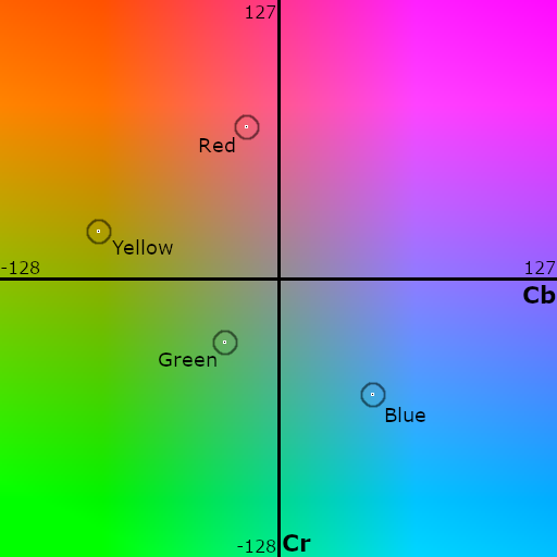
Having the points plotted like so shows how we can identify the individual colours. The algorithm(s) I’m using are shown below:

• max(Cb) –> Blue
• min(Cb) –> Yellow
• max(Cr) –> Red
• min(sqrt(Cr*Cr + Cb*Cb)) (closest to centre) –> Green

As you can see, this identification process is very simple, and should generally not be affected very much by lighting changes, so long as the light is reasonably “white” (after the camera’s white balance correction).

Visiting Corners

Once the corners have been identified, they need to be visited. My first implementation was about as basic as possible:

• Turn to face the corner, using the IMU
• Drive 630 mm straight forwards, counting wheel rotations
• Drive 630 mm straight backwards, counting wheel rotations
• Turn to next corner, repeat

This proved to work pretty well. Over such short distances, and with straight lines, dead-reckoning using wheel rotations is effective. The main downside to this approach is that it can mean driving more distance than strictly required, and spending more time turning, meaning it’s overall slower.

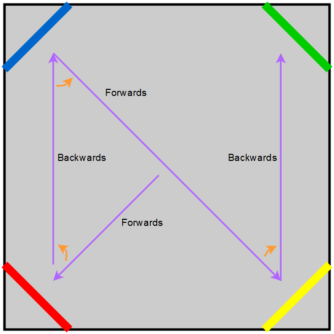
Optimisation

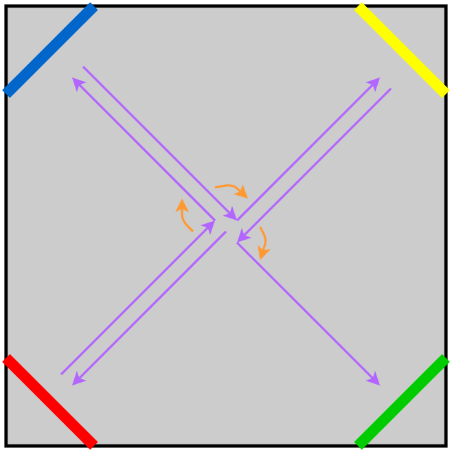
By way of improvement, I implemented a new algorithm which doesn’t go via the centre for each corner, and minimises turning as far as possible. It still only drives in straight lines, but once a corner has been visited, the algorithm determines how best to get to the next corner. There’s two possibilities:

• Next corner is “Adjacent” - drive parallel to the wall
• Next corner is “Opposite” - drive across the centre

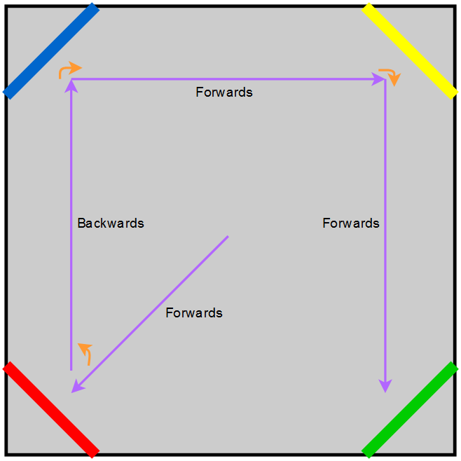
In either case, the code determines how to drive the required course whilst turning the smallest amount possible. Sometimes, this means it will drive backwards, to avoid needing to turn the extra 180°.

With this approach, the time taken depends on how the coloured boards are arranged. In the best case, they are organised already “in-order” - RBYG either clockwise or anticlockwise. In this case, the bot will drive to the first corner, make a 45° turn, and then drive along three sides of the arena making a 90° turn at each corner.

However, there are many other permutations requiring different patterns. The algorithm handles them all, picking the “shortest” route possible.

The last optimisation is to avoid doing the corner scan on every run. The challenge rules state that we should make three runs, and that the colours will be randomised before our first run. That means that once the corners have been identified on the first run, the second and third can skip the initial scanning step and just drive the calculated route. I added support for this, “remembering” the identified order, with a button which can be used to clear the memory if needed.

A “full” run of the final algorithm is shown in the video below.

---

1. Note that the marked points don’t look exactly the same as in the picture of the boards. This is because the ‘Y’ Luma information is ignored. ↩︎