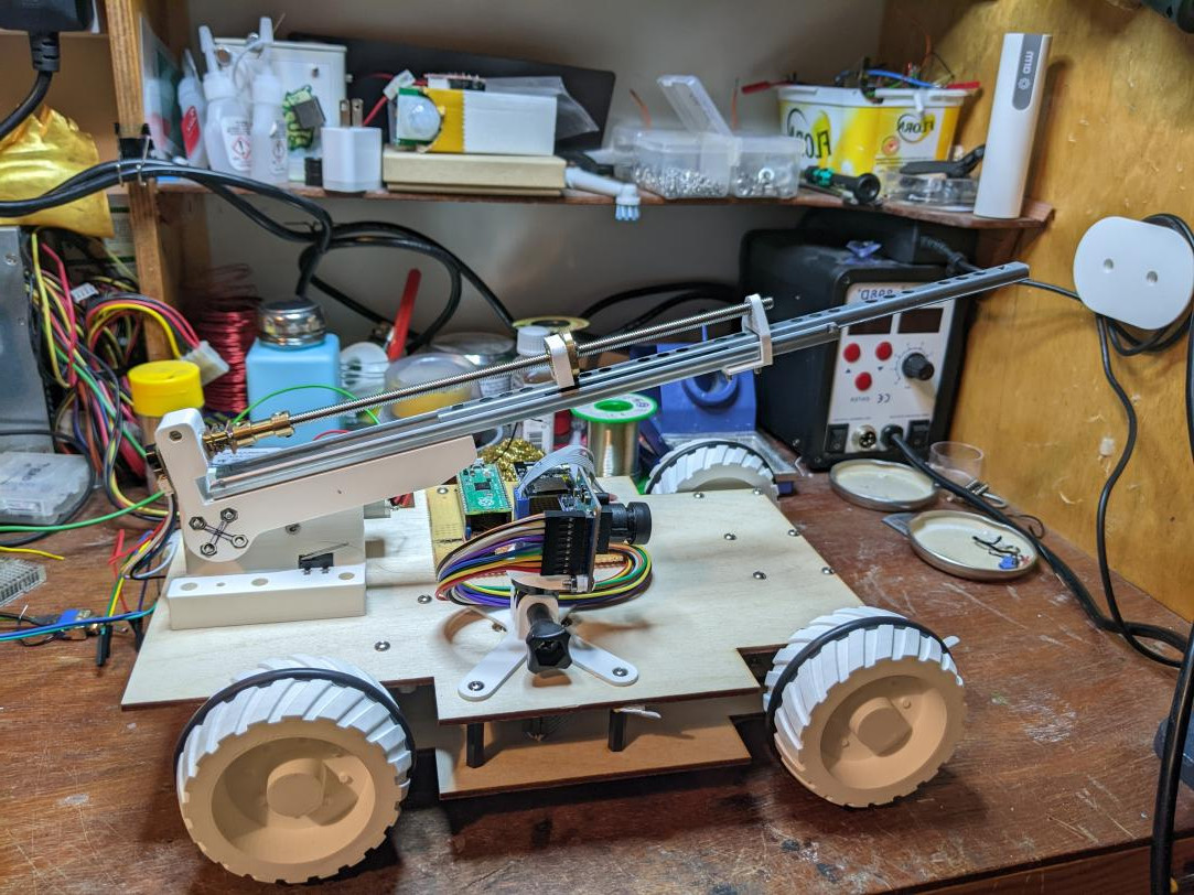
This post is the second in a trilogy detailing the boom on my Pi Wars 2022 robot M0o+.

In the last post, I wrote about the mechanical and electronic design. In this middle post, I’ll be describing the equations which let me find out where the end of the boom is, and next time will go into the equations which let me control where the end of the boom is.

The end goal is to have the ability to say (in code): “move the boom so that the end is 241 mm above the ground and 76 mm in front of the robot,” and then the robot just takes care of all the motor movements to do that. That will form the basis of using the boom to achieve useful work in the challenges.

In-between here and that end goal, we will need to go through some maths; but for the most part we can let a computer take care of the details.

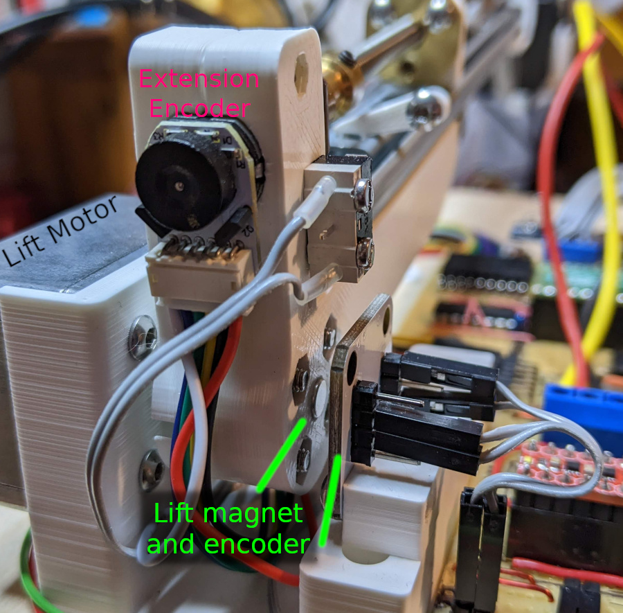
I mirrored this photo so it matches the other diagrams on this page, and seeing my workbench in reverse really messes with my head! 😕

Robot Kinematics

First I need to start with some terminology.

Define: Kinematics (from Wikipedia)

Kinematics is a subfield of physics, developed in classical mechanics, that describes the motion of points, bodies (objects), and systems of bodies (groups of objects) without considering the forces that cause them to move.

The boom on M0o+ can be thought of as a kind of “robotic arm”, or more formally a kinematic chain, which is just a jargon way of saying a bunch of rigid things called links connected by joints which move.

In the field of robot kinematics there’s basically two types of joint:

• A revolute joint is a joint which rotates. Like an elbow, or the hinge in a pair of scissors.
• A prismatic joint is a joint which slides. Like a drawer runner.

In the context of M0o+’s boom, if we ignore the “forks” (which I’m going to do for the majority of this process), there are just two joints:

1. The lift motor forms a revolute joint at the base, which raises and lowers the boom.
2. The drawer runner/leadscrew forms a prismatic joint, which extends and retracts the boom.

At the end of the kinematic chain (at the end of the boom), is the end effector. In my case that’s just where the forks would attach, but for example on an automotive welding robot, that would be where the welding tool is, or the hot end on a 3D printer.

Joint position feedback

To work out where the end effector is, the first step is to find out what the joint positions are. In the case of the revolute “lift” joint, that means “what angle is the boom at?” And in the case of the prismatic “extend” joint that means “how long is the drawer runner?”

As I described in the last post, the “lift” joint has an absolute position magnetic encoder on it, which directly tells me the angle of the boom; and the “extend” leadscrew motor has an encoder which I can use to figure out how extended it is.

This will already be quite a long post, so I won’t go into the details of exactly how I’m handling the sensors, but just take it as given that we can always read the sensors to find out the positions of the two joints at any moment in time.

So that’s position feedback sorted.

Forward Kinematics

Knowing the joint angles is one thing, but what I actually want to know is the position of the end of the boom. Forward kinematics is just the fancy name for working out: “given these joint positions, where is the end effector?”

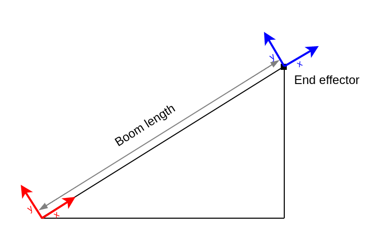
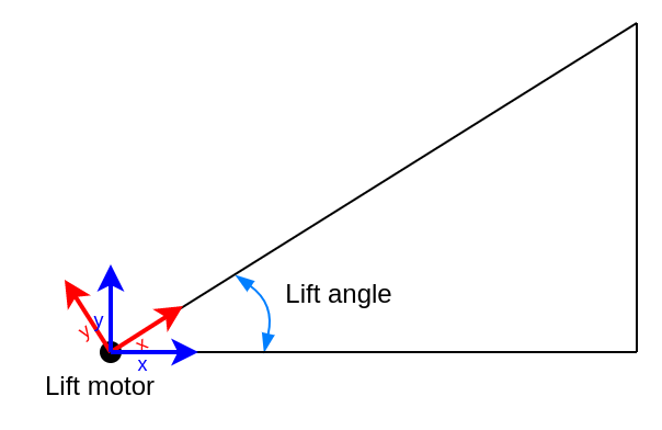
To start with, we can simplify the problem and think about the boom as a right-angled triangle: The hypotenuse represents the boom, with a length equal to the length of the prismatic joint (drawer runner), and the bottom-left corner represents the axle of the lift motor:

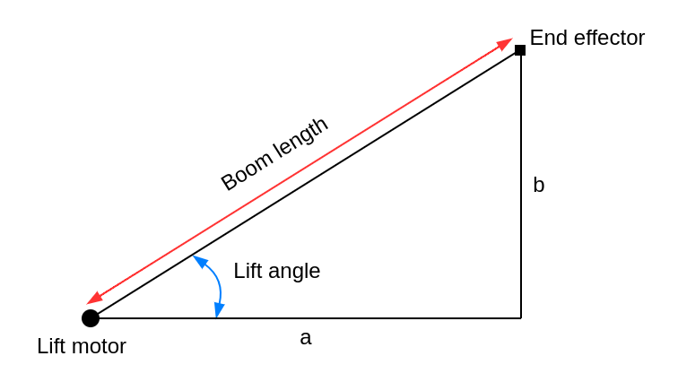
Using some trigonometry, it’s not too hard to see how we can use this to find out the lengths of the other two sides (a and b):

a = boom_length * cos(lift_angle)
b = boom_length * sin(lift_angle)

…and that’s it! We’ve derived the forward kinematics equation(s) for this simple kinematic chain. We can feed the known boom_length and lift_angle values from the sensors into the two equations above, and we’ll get back the a and b positions telling us how far to the right (a) and how far up or down (b) the end of the boom is relative to the motor axle. Great!

Well, not quite

Unfortunately, the real boom isn’t quite a simple triangle. Below is a more accurate sketch, and you can see there are some extra bits I’ve coloured in green which need to be taken into account - there’s an offset from the motor axle to the start of the drawer runner, and there’s the servo mount attached to the far end:

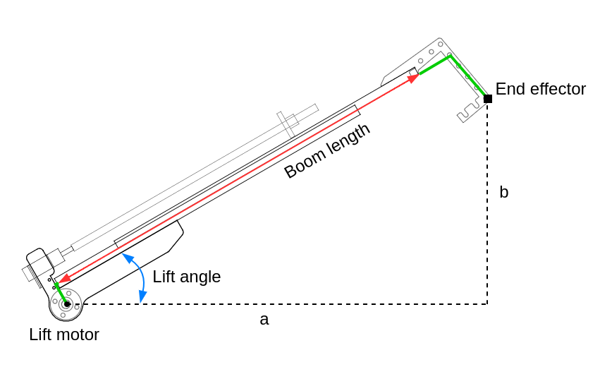
It’s possible to work out the specific geometry by hand take these green bits into account, but when it comes to the inverse kinematics later (in the next post), these extra fiddly bits will make things much more difficult. Instead, there’s a generalised approach which works for all kinds of kinematic chains, from my simple 2-joint boom to an ultra-complex industrial robot arm.

Link Transforms

The basic idea is that we work out a coordinate transformation for each joint of the robot arm boom.

Imagine two teams in a football match. On a compass, North, East, South and West point in the same directions for both teams, that’s the “world” coordinate system. However, each team would have a different idea about which way “forwards” is: that’s the direction towards the other team’s goal. Each team has its own “local” coordinate system. To transform from one team’s “local” coordinate system to the other team’s “local” coordinate system, we need to rotate 180 degrees around the centre spot, and to convert either into “world” coordinates, we need to know which compass direction the pitch faces.

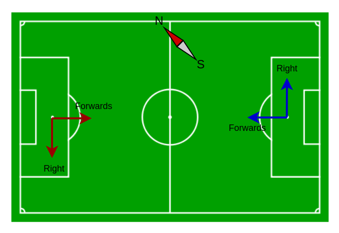
Football pitch image by Paweł Cieśla Staszek Szybki Jest, from Wikimedia Commons

We can think about the robotic arm boom in a similar way. We give each joint its own “local” coordinate system, and we work out the coordinate transformation from one joint to the next. By adding up (actually, multiplying) all of the transformations together, we get one big transformation, which converts from “local” coordinates relative to the end effector into “world” coordinates.

How does that help? Well, coordinate (0, 0) in the “local” coordinate system of the end effector is the coordinate of the end effector itself, so if we have a way to convert from that to a “world” coordinate, we have found the “world” coordinate of the end effector, and that’s exactly what we want 😄

The boom only moves in two dimensions, which makes things a bit simpler. In terms of the diagrams on this page, all of the transformations can be described a rotation around one axis (imagine sticking a pin into the diagram and spinning it around) and a translation left/right and up/down.

Transformation Matrices

Before we go further, I have to introduce transformation matrices.

As with most mathematical Wikipedia pages, that one is pretty hard going, but the important part is that our rotations can be described as a matrix which looks like this (where θ is the rotation angle):

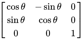
We’ll call that rotation(theta).

And our translations can be described with a matrix which looks like this (where t_x and t_y are the translations left/right and up/down, respectively):

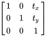
We’ll call that translation(x, y).

We can combine transformations by multiplying the individual matrices together, but it’s backwards (right-to-left), so a translation followed by a rotation would be:

translate_then_rotate = rotation(theta) * translation(x, y)

To actually use a transformation matrix, we multiply it by the point we want to transform:

point_translated_then_rotated = rotation(theta) * translation(x, y) * Matrix([point.x, point.y, 1])

An extra “1” got added as a third coordinate in our 2D point: [point.x, point.y, 1]; if you really want to know why you’ll need to learn about Homogenous Coordinates.

The good news is, we can use Sympy (which is awesome) to take care of all the maths, we just need to remember:

• rotation(theta) means a rotation transformation matrix.
• translation(x, y) means a translation transformation matrix.
• Multiplying transformation matrices together combines their transformations in right-to-left order.

The python code is included at the bottom of this post

Transformations for the simple triangle

To illustrate how the maths works, let’s go back to the simple triangle that we already worked out using basic trigonometry:

a = boom_length * cos(lift_angle)
b = boom_length * sin(lift_angle)

We’ve got two joints, 3 “local” coordinate systems, and so we need to find two coordinate transformations:

1. To transform from coordinates relative to the “start” of the drawer runner to coordinates relative to the “end” of the drawer runner.

This is just a simple translation to the right by boom_length:

translation(boom_length, 0)

2. To transform from coordinates relative to the lift motor axle, to coordinates relative to the “start” of the drawer runner.

This is just a rotation by the lift_angle:

rotation(lift_angle)

Now we can find the combined transformation matrix for both joints by multiplying them together (backwards 😄), and then we can feed in the coordinate (0, 0) to find out the equations for the position of the end of the boom:

>>> combined = rotation(lift_angle) * translation(boom_length, 0)
>>> combined * Matrix([0, 0, 1])
Matrix([
[boom_length*cos(lift_angle)],    # <---- a
[boom_length*sin(lift_angle)],    # <---- b
[                          1]])

How about that! You can see that the result is the same as we worked out by hand earlier!

a = boom_length*cos(lift_angle)
b = boom_length*sin(lift_angle)

Transformations for the real deal

Now that we’ve tested out the maths, we’re going to treat the real boom as having 3 links in the kinematic chain. Starting from the end and working back:

Link 3. The servo mount on the end of the boom.

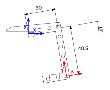
This is the last link, and it’s fixed (there’s no moving joint). We want to transform from coordinates relative to the end of the drawer runner (blue), to coordinates relative to the bottom hole which is where the fork pivot is (red).

The (red) coordinate system here is the “local” coordinate system of the end effector.

The transformation is:

• Translate 30mm to the right
• Translate 48.5mm down
• Rotate anticlockwise 10 degrees (around the “blue” origin)

A3 = rotation(10) * translation(30, -48.5)

Link 2. The drawer runner.

This link has a different transformation depending on the extension of the drawer runner, but it only ever has a translation, there’s no rotation. It transforms from coordinates relative to the start of the runner (red) to coordinates relative to the end of the runner (blue). This is the same as for the triangle example.

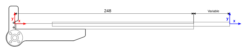
The transformation is:

• Translate to the right by the boom length (variable)

A2 = translation(boom_length, 0)

Link 1. The lift motor

This link transforms from coordinates relative to the lift motor axle (blue), to coordinates relative to the start of the drawer runner (red). This time, the translation is fixed, but the rotation depends on the angle of the lift motor.

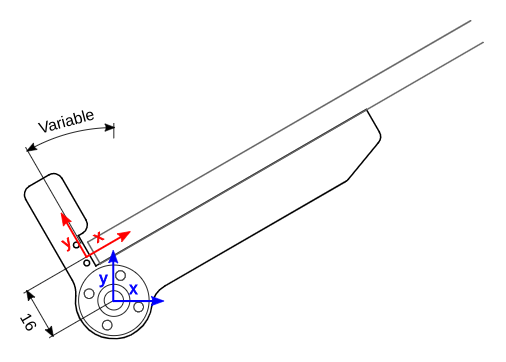
The transformation is:

• Translate up by 16 mm
• Rotate by the lift motor angle (around the lift motor axle)

A1 = rotation(lift_angle) * translation(0, 16)

With transformations found for all the links, they can be combined together the same way as before to find the expressions for a and b:

>>> A3 = rotation(10) * translation(30, -48.5)
>>> A2 = translation(boom_length, 0)
>>> A1 = rotation(lift_angle) * translation(0, 16)
>>> combined = A1 * A2 * A3
>>> combined * Matrix([0, 0, 1])
Matrix([
[boom_length*cos(lift_angle) - 16*sin(lift_angle) - (-48.5*cos(pi/18) + 30*sin(pi/18))*sin(lift_angle) + (48.5*sin(pi/18) + 30*cos(pi/18))*cos(lift_angle)],
[boom_length*sin(lift_angle) + (48.5*sin(pi/18) + 30*cos(pi/18))*sin(lift_angle) + (-48.5*cos(pi/18) + 30*sin(pi/18))*cos(lift_angle) + 16*cos(lift_angle)],
[                                                                                                                                                        1]])

After asking Sympy to simplify the constant terms, we get:

a = boom_length*cos(lift_angle) + 26.55*sin(lift_angle) + 37.97*cos(lift_angle)
b = boom_length*sin(lift_angle) + 37.97*sin(lift_angle) - 26.55*cos(lift_angle)

…which we can use directly in the robot’s code to find a and b for any joint positions read from the sensors, and therefore find the location of the end effector:

As you can see, the “green bits” on the diagram added quite a lot of complexity to the forward kinematics equations.

The really nice thing about this joint transformation approach is that you can very easily make changes to the robot. There’s no need to spend ages trying to work out triangles and congruent angles… you just need to work out the transformation for each link individually, and then get the computer to multiply it all together and spit out the answer.

Next time: Inverse Kinematics

So far all we’ve managed to do is calculate the forward kinematics, converting from joint positions, to end effector coordinates.

What we really want is the opposite - we want to convert from some desired end effector coordinates to the joint positions needed to reach them. That’s called inverse kinematics, and I’ll tackle that in a separate post because this one is already long enough! 😄

Sympy code

Here’s the full python code for the forward kinematics if you want to have a go yourself:

from sympy import *

def deg2rad(degrees):
    return degrees * pi / 180

def rotation(theta):
    return Matrix([
        [ cos(theta), -sin(theta), 0 ],
        [ sin(theta),  cos(theta), 0 ],
        [            0,             0, 1 ],
    ])

def translation(x, y):
    return Matrix([
        [ 1, 0, x ],
        [ 0, 1, y ],
        [ 0, 0, 1 ],
    ])

# Define some variables to use in sympy expressions
lift_angle, boom_length = symbols('lift_angle, boom_length')
x, y = symbols('x, y')

# Calculate the transformations
A3 = rotation(deg2rad(10)) * translation(30, -48.5)
A2 = translation(boom_length, 0)
A1 = rotation(lift_angle) * translation(0, 16)
combined = A1 * A2 * A3

# Find the expressions for the end effector positions
end_effector_pos = combined * Matrix([0, 0, 1])

# Turn the expressions into equations by setting them equal to x and y.
x_eqn = Eq(x, end_effector_pos[0])
y_eqn = Eq(y, end_effector_pos[1])

# Print them
pprint(x_eqn.evalf(4), use_unicode=false)
pprint(y_eqn.evalf(4), use_unicode=false)