Last time, I derived the Forward Kinematics for the boom on M0o+. If you haven’t read the first two posts, then this one won’t make much sense (and I don’t want to repeat myself 😄):

• Part 1: Mechanical and electronic design
• Part 2: Forward Kinematics

This time, we’ll finish off the series by looking at the Inverse Kinematics and actually controlling the boom.

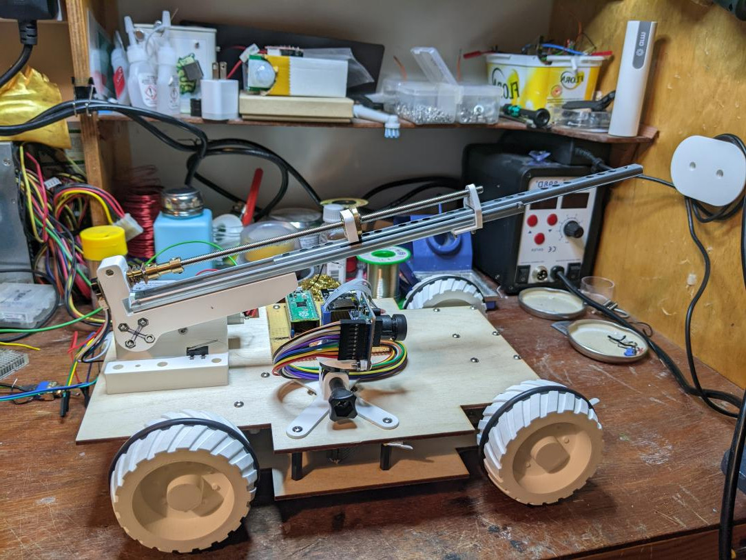
As a quick recap, here’s the basic boom setup. For Inverse Kinematics purposes there are two joints which can move:

1. The lift motor raises and lowers the boom.
2. The drawer runner/leadscrew extends and retracts the boom.

And the end goal is to have the ability to say (in code): “move the boom so that the end is 241 mm above the ground and 76 mm in front of the robot,” and then the robot just takes care of all the motor movements to do that. That will form the basis of using the boom to achieve useful work in the challenges.

Inverse Kinematics summary

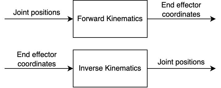
So last time I derived the forward kinematics, which converts from joint positions (lift angle and leadscrew length) to the resulting coordinates of the end of the boom.

What we really want is the opposite - we want to convert from some desired end effector coordinates to the joint positions needed to reach them, and that’s called inverse kinematics.

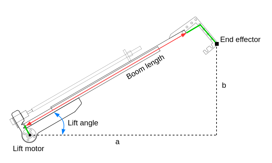
So at the end of the last post, the culmination of all my efforts were two equations which give the “X” and “Y” coordinates (or a and b values in the diagram above):

a = boom_length*cos(lift_angle) + 26.55*sin(lift_angle) + 37.97*cos(lift_angle)
b = boom_length*sin(lift_angle) + 37.97*sin(lift_angle) - 26.55*cos(lift_angle)

To do the opposite, it would be necessary to rearrange these two equations to get two new equations with just lift_angle and boom_length on the left, and just expressions in terms of a and b on the right.

It might be possible to do such a rearrangement “analytically” (using pen and paper, trigonometric identities and all that fun stuff), and I did spend some time trying to do so, but ultimately I failed. So instead, there’s an alternative technique which requires more computation on the robot, and is somewhat approximate, but avoids the need to do this rearrangement by hand.

This excellent document from the University of Illinois was extremely useful to me for working this out. I’m going to focus on the specific implementation for my boom, but if you want some of the more general maths behind it, I’d definitely recommend that page.

The approach in a nutshell

Looking at the diagram below, we can intuitively see that to move from the current position to the target position, the lift angle and boom length both need to increase, so if we were controlling the boom manually we might increase both of them a little bit, and then re-assess the situation:

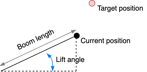
The inverse kinematics is going to do exactly that, with code and maths.

We have a position that we want to move the boom to - let’s call that our “target” position - and we know the current position, which can be found using the forward kinematics equations above.

If we can find a small change in joint positions which moves us towards the target position, then we could move that small amount, getting slightly closer to the target, and then repeat.

The “small change” part means that we need to find a relationship between change in joint position and change in boom coordinates, which in maths speak would mean differentiating our position equation(s) (forward kinematics) with respect to the joint positions.

Partial Differentials and Jacobian Matrices

The whole method depends on something called a Jacobian, which is going to need some school-level maths to explain.

If we have an equation, we can differentiate it with respect to one of its variables, to find out how changing the value of one variable affects the other.

Given the equation:

y = 2x

Differentiating with respect to x gives:

dy/dx = 2

And this tells us that any change in x causes a change in y which is 2 times as big.

If we have an equation with more than two variables, then we can calculate partial derivatives for each of the independent variables in turn, treating the other independent variables as if they are constants.

The equation:

z = 2x + 3y

Has the partial derivative with respect to x:

Note that we treat y as a constant, so 3y has a derivative of 0.

dz/dx = 2 + 0

And with respect to y of:

dz/dy = 0 + 3

These tell us how much z changes for each change in x and y respectively. However, note that because we treated the “other” variable as a constant, these partial derivatives only hold true for a constant value of the “other” variable.

If we took one of the forward kinematics equations, then we can find its partial derivatives with respect to the two independent variables: lift_angle and boom_length.

a = boom_length*cos(lift_angle) + 26.55*sin(lift_angle) + 37.97*cos(lift_angle)

da/dlift_angle = -boom_length*sin(lift_angle) + 26.55*cos(lift_angle) - 37.07*sin(lift_angle)

da/dboom_length = cos(lift_angle)

This isn’t so obvious unless you’ve got a lot of practice calculating derivatives, but you don’t have to work it through by hand if you don’t want to: we can get sympy to do it for us!

>>> a
boom_length*cos(lift_angle) + 26.55*sin(lift_angle) + 37.97*cos(lift_angle)
>>> diff(a, lift_angle)
-boom_length*sin(lift_angle) - 37.97*sin(lift_angle) + 26.55*cos(lift_angle)
>>> diff(a, boom_length)
cos(lift_angle)

Magical!

Now, a Jacobian Matrix is the name for a matrix containing the partial differentials of a set of functions with respect to their independent variables, like the a and b functions that we got from forward kinematics.

Sticking with our equation for a, the Jacobian of a would be a matrix with one row, where each column is one of the partial differentials from above (Using sympy syntax, because who wants to do calculus when the computer can do it for us?):

J_a = [ diff(a, lift_angle), diff(a, boom_length) ]

We actually have two equations, one for a and one for b, so we can get a combined Jacobian, where the first row has the partial differentials for a and the second row, for b:

J = Matrix([
	[ diff(a, lift_angle), diff(a, boom_length) ],
	[ diff(b, lift_angle), diff(b, boom_length) ],
])

…and that’s all a Jacobian is.

How does this help?

Well, the partial differentials tell us what change we can expect in a or b if we change lift_angle or boom_length. This is exactly the “relationship between change in joint position and change in boom coordinates” I mentioned before.

More concretely, if we take our Jacobian and multiply by a vector containing changes in joint positions, we will get back changes in coordinates:

[ change_in_a, change_in_b ]' = J * [change_in_lift_angle, change_in_boom_length]'

Things can get a bit confusing here with all the different variables. To actually use the equation above, you would:

1. Calculate the Jacobian matrix, filling in the known values for the current lift_angle and boom_length
2. Pick some small values for change_in_lift_angle and change_in_boom_length and feed them in to the equation
3. Calculate change_in_a and change_in_b according to the equation.

Step 1 is crucially important here - the Jacobian matrix depends on lift_angle and boom_length, and so it must be recalculated for each new lift_angle and boom_length.

The inverse part

OK, so all the derivation above gave us an equation which lets us calculate change in boom coordinates, given a current position and a change in joint positions.

Once again, we still want the opposite of that: an equation that calculates the required changes in joint positions, given a desired change in boom position.

We know the desired change in boom position - that’s target_position - current_position, what we want to calculate is the required change in joint positions.

To get that, we “simply” invert the Jacobian, which results in an equation like so:

[ change_in_lift_angle, change_in_boom_length ]' = J.inv() * [ desired_change_in_a, desired_change_in_b ]'

For inverting the Jacobian, we just use the standard 2x2 matrix inverse equation.

Putting that into code

That’s all the derivation done, to actually use it on the robot looks something like this:

while target_position_not_reached():
	# Get the current position
	current_lift, current_length = get_current_joint_positions()

	# Calculate Jacobian
	jacobian = calculate_jacobian(current_lift, current_length)
	inv_jacobian = invert(jacobian)

	# Find out the desired change in end effector position
	[d_a, d_b] = target_position - current_position

	# Find an approximation for the change in joint positions needed
	[d_lift, d_length] = inv_jacobian * [d_a, d_b]

	# Move a little in the right direction
	move_lift_motor_towards(current_lift + d_lift)
	move_extend_towards(current_length + d_length)
	wait_a_short_time()

Because the calculated Jacobian only applies for those specific values of current_lift and current_length, the d_lift and d_length values are approximations - as soon as the joints move, the Jacobian needs recalculating, and we need to recalculate new d_lift and d_length values. That’s what the wait_a_short_time() is there for; we wait for the boom to move a little bit, and then recalculate.

And that’s the basis of a forward kinematics solution for my boom.

Trajectory planning

The implementation above is always going to try and move directly towards the target position, but what I found was due to the approximate nature of the calculations, and because I don’t have anything like perfect speed control for the joints, the boom would move to the correct position, but it wouldn’t move there in a straight line.

This can be a problem - it can mean that the boom bashes into something (like the apple tree) because the lift motor moved more quickly than the extension motor could keep up, or vice-versa.

To fix this, I added a trajectory planner. The trajectory planner doesn’t only keep track of the current position and the target position, it also keeps track of the starting position.

Then, instead of setting the inverse kinematics to move directly to the target position, it sets a bunch of intermediate targets along the path from the start to the end position.

In summary the trajectory planner does:

1. Get the current boom position
2. Find the point on the intended path closest to the current position
3. Calculate an intermediate target point a small distance further along the intended path from 2.
4. Set the inverse kinematics target to 3.
5. Repeat!

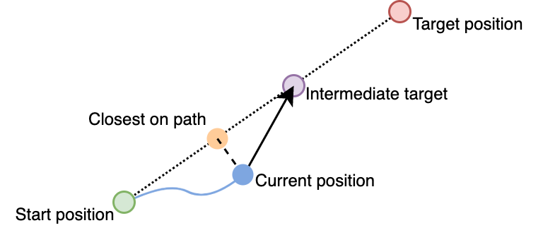
This means that even if the boom moves away from the intended path, the trajectory planner will try and drag it back along the intended path.

Even with this, the boom still doesn’t follow the intended path completely, because the intermediate targets are always on the intended path, the system tends to under-correct; but it works well enough.

Conclusion

So that’s the somewhat complicated process of implementing an inverse kinematics controller for the boom position. With all that in place, I can now tell the boom to move to a target position in the real world (relative to the robot), and the inverse kinematics code will move the two joint motors to get the boom to move to that position.

So next, it’s time to solve some of the actual competition challenges!