Identifying edges is one of the key “features” of the human vision system. Our brains have evolved to identify edges and it’s one of the things which lets us pick out different objects in the world. If we want to teach our computers to see, Edge Detection is one of the key tools needed to reach that goal (at least, according to “classical” methods. Things change with Deep Learning).

Unfortunately, edge detection can be a difficult problem to solve in software. The Wikipedia article has a lot of useful background and insights.

The de-facto standard algorithm for edge detection is called the Canny edge detector algorithm, named after its inventor John F. Canny. This algorithm has proven to be highly versatile, delivering a good balance of performance and complexity.

OpenCV has a Canny implementation, but I decided to eschew use of OpenCV as I found it too easy to completely blow my processing budget with its vast array of powerful algorithms. I also thought I’d learn more by implementing my own computer vision routines.

Efficiently implementing the Canny algorithm is quite an undertaking - but thankfully for the Pi Wars challenges I don’t really need a fully flexible edge detector. All that’s needed (at least for my approaches to the challenges) is finding horizontal and vertical lines between regions of flat, solid colour. That’s a much easier problem to solve!

All of the code described on this page can be found at https://github.com/usedbytes/mini_mouse-cv

Finding Edges

At the most basic level, an edge is just a sharp change in colour. So, if we want to find edges, the first thing that’s needed is to calculate differences in color. That in itself is a hard problem with a lot of nuances.

Minor detour into YUV

I’ve elected to use the YCbCr/YUV colour space, as it has some nice properties:

• Firstly, it separates lightness from colour. That removes a lot of redundancy - meaning that the Cb (U) and Cr (V) channels contain most of the relevant information. Whereas in RGB we often need to look at the value of all three channels to get useful information, in YCbCr, we can often get away with just two. That’s a nice simplification!
  • HSV is another popular colour space which separates lightness from colour - but it has a significant limitation when used for computer vision. Namely, the “hue” of black/grey/white varies wildly, because when saturation is close to zero, hue can be anything without changing the colour. That leads to a very “speckly” hue channel on areas of black or grey.
• Secondly, if we only want greyscale (like I’m using for line following), we can just take the ‘Y’ channel and simply ignore Cb and Cr
• Thirdly it’s natively supported by all kinds of image processing hardware, as it’s the colour space used for effectively all videos. We can get YCbCr data directly out of the Pi’s camera hardware, without needing to do an expensive conversion in software.

In YCbCr, a reasonable color difference algorithm is to just treat it as a 3D cartesian co-ordinate system, and calculate the difference between the two points.

func absdiff_uint8(a, b uint8) int {
	if a < b {
		return int(b - a)
	} else {
		return int(a - b)
	}
}

func DeltaCYCbCr(a, b color.YCbCr) uint8 {
	yDiff := float64(absdiff_uint8(a.Y, b.Y)) / 255.0
	cbDiff := float64(absdiff_uint8(a.Cb, b.Cb)) / 255.0
	crDiff := float64(absdiff_uint8(a.Cr, b.Cr)) / 255.0
	return uint8(math.Sqrt(yDiff * yDiff + cbDiff * cbDiff + crDiff * crDiff) * 255.0)
}

That DeltaCYCbCr() function is the basic building block for comparing pixels.

Horizontal and Vertical Lines

I want to find edges for two very specific purposes. For the Canyons of Mars (maze), I want to find horizontal lines, to find the horizon to tell me how far away from a wall I am. For the Hubble Telescope Nebula Challenge (rainbow), I want to find vertical lines to identify the edges of the coloured boards. Being able to focus only on horizontal and vertical lines makes implementing my own algorithm entirely feasible.

For the rest of this post, I’m going to focus on vertical lines, but the techniques are equally applicable to horizontal lines - just swap “columns” for “rows”.

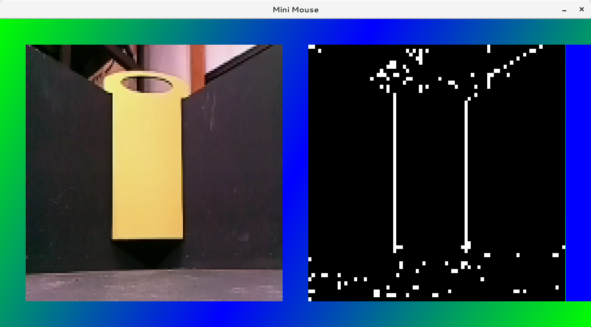
If there’s a vertical edge, we expect a change in color between one pixel and the pixel to its right. The picture below shows the original image, alongside the result of calling DeltaCYCbCr() on each pair of horizontally adjacent pixels (there’s a minor detail I don’t want to dwell on - the resolution of the difference image is halved, due to chroma subsampling).

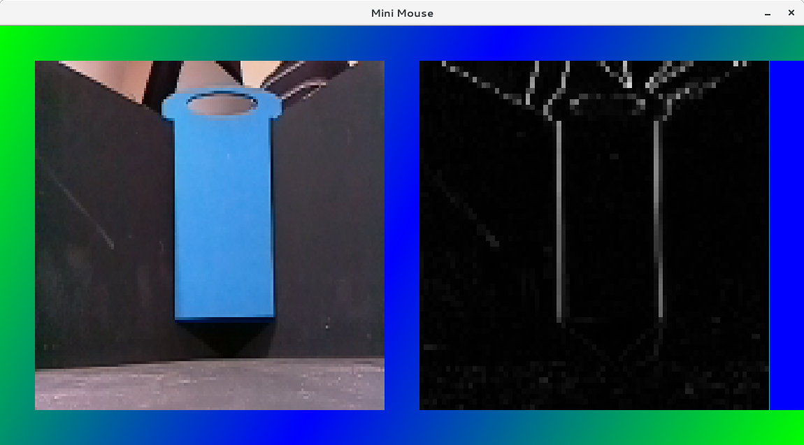
That’s already looking pretty good! This edge detection business isn’t so bad! So this gives us “whiter” pixels along edges, but how to turn that into a location of a line which I can actually use in my program?

First, I use the same thresholding as before, to amplify the strong edges and drop the weak ones.

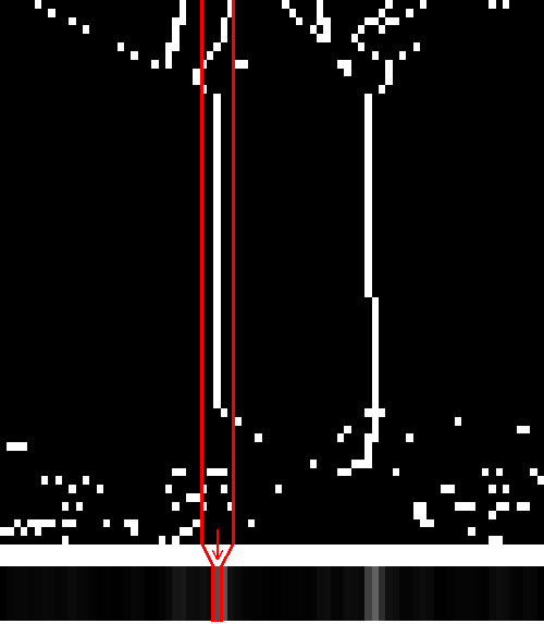
After that, I want to find the columns which have the most white pixels in, because they represent vertical lines. It’s not ideal to just look at individual columns, because if the line isn’t perfectly vertical, its edges are likely to be spread across multiple columns, and we might miss it. Instead, I aggregate the sums of white pixels in vertical stripes of the image, effectively “spreading out” the search window. In the picture below, each column in the bar at the bottom represents the sum of white pixels in the stripe of pixels above it (red lines showing an example for one “stripe”) .

The last step, is to take that row of summed up pixels, and threshold it (I’m really getting good mileage out of that threshold code!), giving me nice clean white spots in the columns which represent the strongest vertical lines.

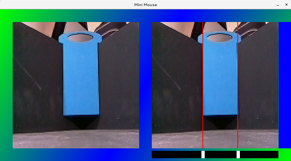
That concludes the basis of line detection. Of course, in this case the input image is quite “kind”, and there’s not a lot of extraneous content to confuse the algorithm. This isn’t the case in general, and so for both the maze and rainbow challenges, I have some specific extra enhancements to make them more robust in the case of less-than-ideal conditions (i.e. the real world). Those will be covered in separate posts.